Preprocessing and clustering 3k PBMCs ¶

This template demonstrates how to use LaminDB to track data provenance and manage artifacts during a standard single-cell RNA-seq analysis workflow. Adapted from the classic Scanpy PBMC3k tutorial, it has additional code showing how to track the notebook’s execution, save the raw dataset as an artifact, and register the final annotated dataset in your LaminDB instance.

We will process a dataset of 3k PBMCs from a Healthy Donor (freely available from 10x Genomics).

Note: To run examples, if you don’t have a LaminDB instance, create one:

!lamin init --storage ./test-pbmc3k

from __future__ import annotations

import matplotlib.pyplot as plt
import pandas as pd
import scanpy as sc
import lamindb as ln

Track the notebook’s execution in LaminDB

ln.track()

Download and unpack the data.

%%bash
mkdir -p data
cd data
test -f pbmc3k_filtered_gene_bc_matrices.tar.gz || curl https://cf.10xgenomics.com/samples/cell/pbmc3k/pbmc3k_filtered_gene_bc_matrices.tar.gz -o pbmc3k_filtered_gene_bc_matrices.tar.gz
tar -xzf pbmc3k_filtered_gene_bc_matrices.tar.gz

  % Total    % Received % Xferd  Average Speed   Time    Time     Time  Current

                              Dload  Upload   Total   Spent    Left  Speed

  0     0    0     0    0     0      0      0 --:--:-- --:--:-- --:--:--     0

100 7443k  100 7443k    0     0  28.4M      0 --:--:-- --:--:-- --:--:-

- 28.5M

Read in the count matrix into an AnnData object.

adata = sc.read_10x_mtx(
    "data/filtered_gene_bc_matrices/hg19/",  # the directory with the `.mtx` file
    var_names="gene_symbols",  # use gene symbols for the variable names (variables-axis index)
    cache=True,  # write a cache file for faster subsequent reading
)
adata

Save the AnnData object with the raw/unprocessed 3k PBMCs in LaminDB¶

ln.Artifact.from_anndata(adata, key="raw_pbmc3k.h5ad").save()

Preprocessing¶

Load the Anndata object with the raw/unprocessed 3k PBMCs from LaminDB¶

adata = ln.Artifact.get(key="raw_pbmc3k.h5ad").load()

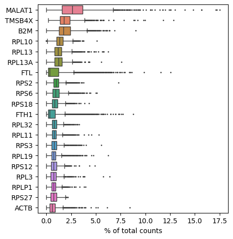
Show those genes that yield the highest fraction of counts in each single cell, across all cells.

sc.pl.highest_expr_genes(adata, n_top=20)

Basic filtering:

sc.pp.filter_cells(adata, min_genes=200)
sc.pp.filter_genes(adata, min_cells=3)
adata

Let’s assemble some information about mitochondrial genes, which are important for quality control.

# annotate the group of mitochondrial genes as "mt"
adata.var["mt"] = adata.var_names.str.startswith("MT-")
sc.pp.calculate_qc_metrics(adata, qc_vars=["mt"], percent_top=None, log1p=False, inplace=True)

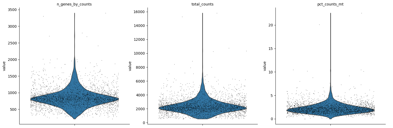
A violin plot of some of the computed quality measures:

the number of genes expressed in the count matrix
the total counts per cell
the percentage of counts in mitochondrial genes

sc.pl.violin(
    adata,
    ["n_genes_by_counts", "total_counts", "pct_counts_mt"],
    jitter=0.4,
    multi_panel=True,
)

Remove cells that have too many mitochondrial genes expressed or too many total counts. Do the filtering by slicing the AnnData object.

adata = adata[
    (adata.obs.n_genes_by_counts < 2500) & (adata.obs.n_genes_by_counts > 200) & (adata.obs.pct_counts_mt < 5),
    :,
].copy()
adata.layers["counts"] = adata.X.copy()
adata

Total-count normalize (library-size correct) the data matrix $\mathbf{X}$ to 10,000 reads per cell, so that counts become comparable among cells.

sc.pp.normalize_total(adata, target_sum=1e4)

Logarithmize the data.

sc.pp.log1p(adata)

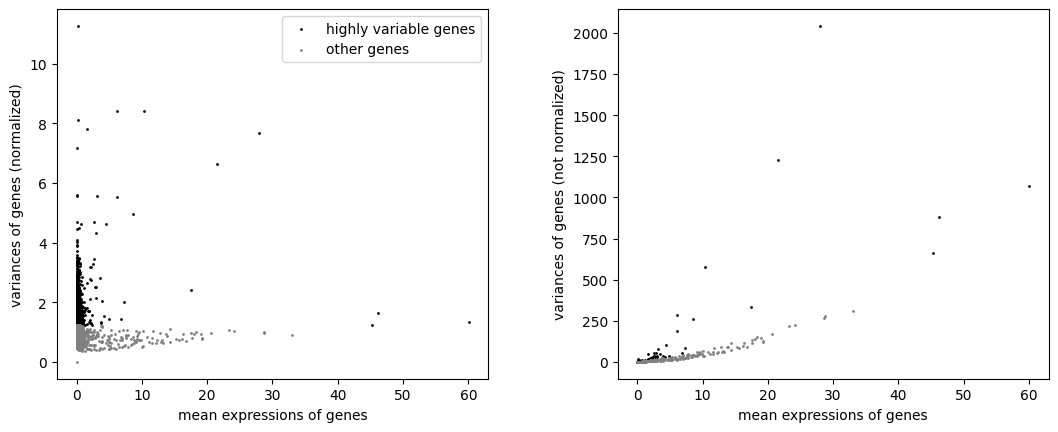
Identify highly-variable genes.

sc.pp.highly_variable_genes(
    adata,
    layer="counts",
    n_top_genes=2000,
    min_mean=0.0125,
    max_mean=3,
    min_disp=0.5,
    flavor="seurat_v3",
)

sc.pl.highly_variable_genes(adata)

Scale each gene to unit variance. Clip values exceeding standard deviation 10.

adata.layers["scaled"] = adata.X.toarray(order='C')
sc.pp.regress_out(adata, ["total_counts", "pct_counts_mt"], layer="scaled")
sc.pp.scale(adata, max_value=10, layer="scaled")

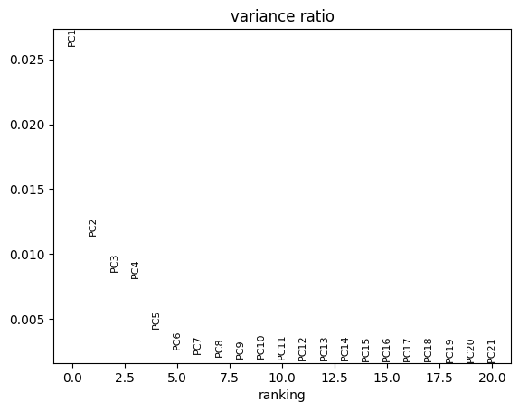
Principal component analysis¶

Reduce the dimensionality of the data by running principal component analysis (PCA), which reveals the main axes of variation and denoises the data.

sc.pp.pca(adata, layer="scaled", svd_solver="arpack")

Let us inspect the contribution of single PCs to the total variance in the data. This gives us information about how many PCs we should consider in order to compute the neighborhood relations of cells, e.g. used in the clustering function sc.tl.louvain() or tSNE sc.tl.tsne().

sc.pl.pca_variance_ratio(adata, n_pcs=20)

Computing the neighborhood graph¶

Compute the neighborhood graph of cells using the PCA representation of the data matrix.

sc.pp.neighbors(adata, n_neighbors=10, n_pcs=40)

Clustering the neighborhood graph¶

sc.tl.leiden(
    adata,
    resolution=0.7,
    random_state=0,
    flavor="igraph",
    n_iterations=2,
    directed=False,
)
adata.obs["leiden"] = adata.obs["leiden"].copy()
adata.uns["leiden"] = adata.uns["leiden"].copy()

Embedding the neighborhood graph in a UMAP¶

sc.tl.paga(adata)
sc.pl.paga(adata, plot=False)  # remove `plot=False` if you want to see the coarse-grained graph
sc.tl.umap(adata, init_pos='paga')
sc.tl.umap(adata)

adata.obsm["X_umap"] = adata.obsm["X_umap"].copy()
sc.pl.umap(adata, color=["leiden", "CD14", "NKG7"])

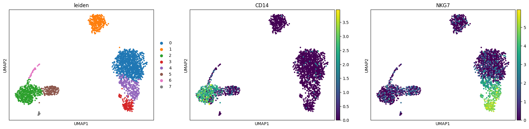
Finding marker genes¶

Let us compute a ranking for the highly differential genes in each cluster.

sc.tl.rank_genes_groups(adata, "leiden", mask_var="highly_variable", method="wilcoxon")
sc.pl.rank_genes_groups(adata, n_genes=25, sharey=False)

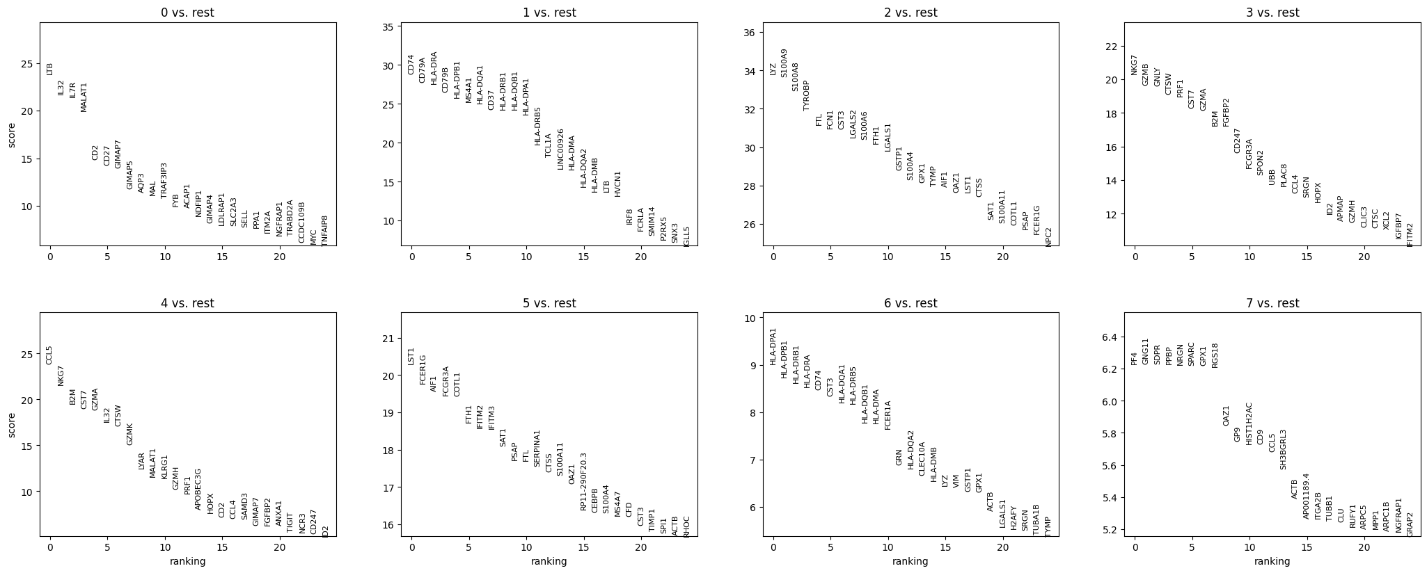
Most of these genes are found in the highly expressed genes with notable exceptions like CD8A (see the below dotplot).

Leiden Group	Markers	Cell Type
0	IL7R	CD4 T cells
1	CD14, LYZ	CD14+ Monocytes
2	MS4A1	B cells
3	CD8A	CD8 T cells
4	GNLY, NKG7	NK cells
5	FCGR3A, MS4A7	FCGR3A+ Monocytes
6	FCER1A, CST3	Dendritic Cells
7	PPBP	Megakaryocytes

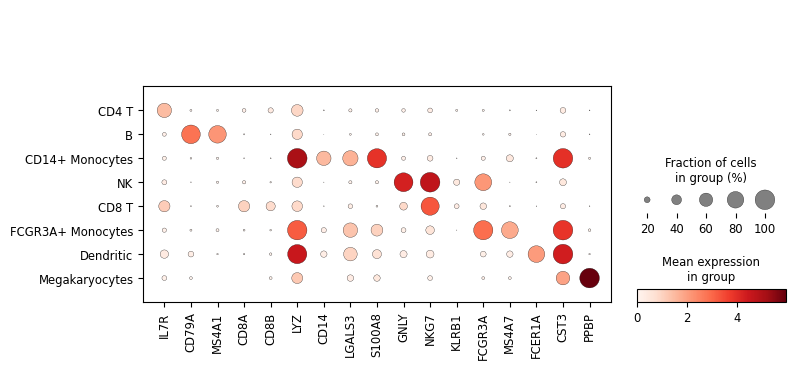
Let us also define a list of marker genes for later reference.

marker_genes = [
    *["IL7R", "CD79A", "MS4A1", "CD8A", "CD8B", "LYZ", "CD14"],
    *["LGALS3", "S100A8", "GNLY", "NKG7", "KLRB1"],
    *["FCGR3A", "MS4A7", "FCER1A", "CST3", "PPBP"],
]

Actually mark the cell types.

new_cluster_names = [
    "CD4 T",
    "B",
    "CD14+ Monocytes",
    "NK",
    "CD8 T",
    "FCGR3A+ Monocytes",
    "Dendritic",
    "Megakaryocytes",
]
adata.rename_categories("leiden", new_cluster_names)
adata.obs['cell_type']=adata.obs['leiden']
adata

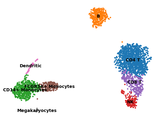
Visualize the cell types in a UMAP

sc.pl.umap(adata, color="cell_type", legend_loc="on data", title="", frameon=False)

Now that we annotated the cell types, let us visualize the marker genes.

sc.pl.dotplot(adata, marker_genes, groupby="cell_type")

Save the resulting AnnData object in LaminDB¶

ln.Artifact.from_anndata(adata, key="result_pbmc3k.h5ad").save()

ln.finish() marks the successful completion of the current script or notebook run in LaminDB, finalizing its execution state and saving the source code to the database for reproducibility.

ln.finish()