Spatial RNA-seq

Here, you’ll learn how to manage spatial datasets:

1. query & analyze spatial datasets ()

2. create and share interactive visualizations with vitessce ()

3. curate and ingest spatial data ()

4. load the collection into memory & train a ML model ()

Spatial omics data integrates molecular profiling (e.g., transcriptomics, proteomics) with spatial information, preserving the spatial organization of cells and tissues. It enables high-resolution mapping of molecular activity within biological contexts, crucial for understanding cellular interactions and microenvironments.

Many different spatial technologies such as multiplexed imaging, spatial transcriptomics, spatial proteomics, whole slide imaging, spatial metabolomics, and 3D tissue reconstruction exist which can all be stored in the SpatialData data framework. For more details we refer to the original publication:

Marconato, L., Palla, G., Yamauchi, K.A. et al. SpatialData: an open and universal data framework for spatial omics. Nat Methods 22, 58–62 (2025). https://doi.org/10.1038/s41592-024-02212-x

Note

A collection of curated spatial datasets in SpatialData format is available on the scverse/spatialdata-db instance.

spatial data vs SpatialData terminology

When we mention spatial data, we refer to data from spatial assays, such as spatial transcriptomics or proteomics, that includes spatial coordinates to represent the organization of molecular features in tissue. When we refer SpatialData, we mean spatial omics data stored in the scverse SpatialData framework.

Query and analyze spatial data

# pip install lamindb spatialdata spatialdata-plot squidpy
!lamin init --storage ./test-spatial --modules bionty

Show code cell output Hide code cell output

→ initialized lamindb: testuser1/test-spatial

import warnings

warnings.filterwarnings("ignore")

import lamindb as ln
import scanpy as sc
import spatialdata as sd
import spatialdata_plot as pl
import squidpy as sq
from matplotlib import pyplot as plt

ln.track()

Show code cell output Hide code cell output

→ connected lamindb: testuser1/test-spatial

→ created Transform('doAyYhzetMh40000', key='spatial.ipynb'), started new Run('2Q17Xrf4RXz9E6Cy') at 2026-01-03 11:52:53 UTC

→ notebook imports: lamindb==1.17.0 matplotlib==3.10.8 scanpy==1.11.5 spatialdata-plot==0.2.13 spatialdata==0.6.1 squidpy==1.7.0

• recommendation: to identify the notebook across renames, pass the uid: ln.track("doAyYhzetMh4")

Query by biological metadata

We’ll work with a human lung cancer dataset generated using 10x Genomics Xenium platform and available in a public instance. This FFPE (formalin-fixed paraffin-embedded) tissue sample includes spatial gene expression profiles.

Create the central query object of our public lamindata instance:

db = ln.DB("laminlabs/lamindata")

Now query the database to find Xenium datasets from lung tissue:

all_xenium_data = db.Artifact.filter(
    assay="Xenium Spatial Gene Expression", tissue="lung"
)

all_xenium_data.to_dataframe()

Show code cell output Hide code cell output

	uid	key	description	suffix	kind	otype	size	hash	n_files	n_observations	version	is_latest	is_locked	created_at	branch_id	space_id	storage_id	run_id	schema_id	created_by_id
id
12608	8sPWscz3SICG1D8t0001	xenium/2.0.0/Xenium_V1_humanLung_Cancer_FFPE_o...	None	.zarr	None	spatialdata	7045222972	jgalhtHw00CzuZA_jrTygw	1457	None	None	True	False	2025-12-16 14:14:28.067901+00:00	1	1	2	None	None	40

Analyze spatial data

sdata = all_xenium_data[0].load()

Show code cell output Hide code cell output

no parent found for <ome_zarr.reader.Label object at 0x7f861e1928a0>: None

no parent found for <ome_zarr.reader.Label object at 0x7f861e512900>: None

→ transferred: Artifact(uid='8sPWscz3SICG1D8t0001'), Storage(uid='D9BilDV2')

Spatial data datasets stored as SpatialData objects can easily be examined and analyzed through the SpatialData framework, squidpy, and scanpy.

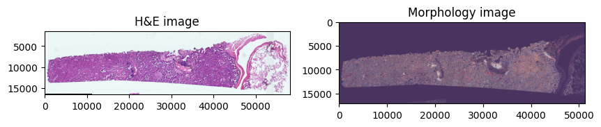
We use spatialdata-plot to get an overview of the dataset:

axes = plt.subplots(1, 2, figsize=(10, 10))[1].flatten()
sdata.pl.render_images("he_image", scale="scale4").pl.show(
    ax=axes[0], title="H&E image"
)
sdata.pl.render_images("morphology_focus", scale="scale4").pl.show(
    ax=axes[1], title="Morphology image"
)

INFO     Your image has 5 channels. Sampling categorical colors and using multichannel strategy 'stack' to render. 

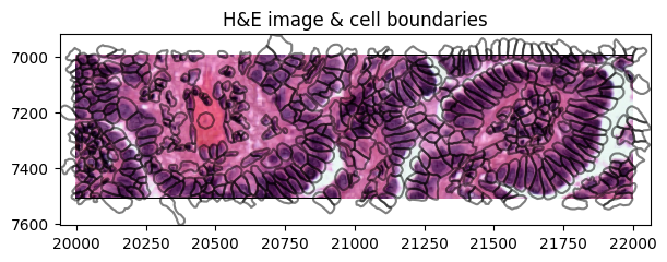
We can visualize the segmentations masks by rendering the shapes from the SpatialData object:

def crop0(x):
    return sd.bounding_box_query(
        x,
        min_coordinate=[20000, 7000],
        max_coordinate=[22000, 7500],
        axes=("x", "y"),
        target_coordinate_system="global",
    )


crop0(sdata).pl.render_images("he_image", scale="scale2").pl.render_shapes(
    "cell_boundaries", fill_alpha=0, outline_alpha=0.5
).pl.show(
    figsize=(10, 5), title="H&E image & cell boundaries", coordinate_systems="global"
)

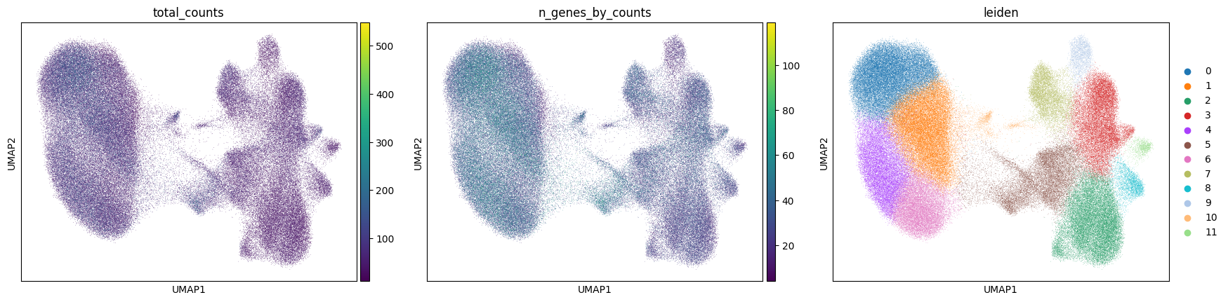
For any Xenium analysis we would use the AnnData object, which contains the count matrix, cell and gene annotations. It is stored in the spatialdata.tables slot:

adata = sdata.tables["table"]
adata

Show code cell output Hide code cell output

AnnData object with n_obs × n_vars = 154472 × 377
    obs: 'cell_id', 'transcript_counts', 'control_probe_counts', 'control_codeword_counts', 'unassigned_codeword_counts', 'deprecated_codeword_counts', 'total_counts', 'cell_area', 'nucleus_area', 'region', 'z_level', 'nucleus_count', 'cell_labels', 'n_genes_by_counts', 'log1p_n_genes_by_counts', 'log1p_total_counts', 'pct_counts_in_top_10_genes', 'pct_counts_in_top_20_genes', 'pct_counts_in_top_50_genes', 'pct_counts_in_top_150_genes', 'n_counts', 'leiden'
    var: 'gene_ids', 'feature_types', 'genome', 'n_cells_by_counts', 'mean_counts', 'log1p_mean_counts', 'pct_dropout_by_counts', 'total_counts', 'log1p_total_counts', 'n_cells'
    uns: 'spatialdata_attrs', 'umap', 'neighbors', 'leiden', 'log1p', 'pca'
    obsm: 'spatial', 'X_pca', 'X_umap'
    varm: 'PCs'
    layers: 'counts'
    obsp: 'connectivities', 'distances'

adata.obs

Show code cell output Hide code cell output

	cell_id	transcript_counts	control_probe_counts	control_codeword_counts	unassigned_codeword_counts	deprecated_codeword_counts	total_counts	cell_area	nucleus_area	region	z_level	nucleus_count	cell_labels	n_genes_by_counts	log1p_n_genes_by_counts	log1p_total_counts	pct_counts_in_top_10_genes	pct_counts_in_top_20_genes	pct_counts_in_top_50_genes	pct_counts_in_top_150_genes	n_counts	leiden
1	aaaaficg-1	19	0	0	0	0	19.0	49.130002	21.268595	cell_circles	0.0	1.0	2	15	2.772589	2.995732	73.684211	100.000000	100.000000	100.0	19.0	2
2	aaabbaka-1	53	0	0	0	0	53.0	119.618911	74.778753	cell_circles	0.0	1.0	3	38	3.663562	3.988984	45.283019	66.037736	100.000000	100.0	53.0	1
3	aaabbjoo-1	29	0	0	0	0	29.0	94.241097	59.109533	cell_circles	0.0	1.0	4	18	2.944439	3.401197	72.413793	100.000000	100.000000	100.0	29.0	0
4	aaablchg-1	42	0	0	1	0	42.0	120.341411	52.426408	cell_circles	0.0	1.0	5	33	3.526361	3.761200	45.238095	69.047619	100.000000	100.0	42.0	1
5	aaacaicl-1	135	0	0	0	0	135.0	197.965007	56.084065	cell_circles	0.0	2.0	6	62	4.143135	4.912655	50.370370	68.888889	91.111111	100.0	135.0	1
...	...	...	...	...	...	...	...	...	...	...	...	...	...	...	...	...	...	...	...	...	...	...
162244	oipogjpd-1	12	0	0	0	0	12.0	6.818594	6.818594	cell_circles	7.0	1.0	162245	12	2.564949	2.564949	83.333333	100.000000	100.000000	100.0	12.0	11
162245	oipoiane-1	11	0	0	0	0	11.0	13.140469	13.140469	cell_circles	6.0	1.0	162246	9	2.302585	2.484907	100.000000	100.000000	100.000000	100.0	11.0	2
162246	oipolbma-1	10	0	0	0	0	10.0	34.634845	8.940938	cell_circles	5.0	1.0	162247	10	2.397895	2.397895	100.000000	100.000000	100.000000	100.0	10.0	5
162247	oippajff-1	13	0	0	0	0	13.0	33.731720	5.644531	cell_circles	7.0	1.0	162248	13	2.639057	2.639057	76.923077	100.000000	100.000000	100.0	13.0	2
162248	ojaacmoj-1	11	0	0	0	0	11.0	14.540313	14.540313	cell_circles	5.0	1.0	162249	10	2.397895	2.484907	100.000000	100.000000	100.000000	100.0	11.0	7

154472 rows × 22 columns

Quality control metrics can be calculated using scanpy.pp.calculate_qc_metrics. Cells and genes can be filtered based on minimum thresholds using scanpy.pp.filter_cells and scanpy.pp.filter_genes.

For normalization and dimensionality reduction, standard scanpy workflows include:

• scanpy.pp.normalize_total for library size normalization

• scanpy.pp.log1p for log transformation

• scanpy.pp.pca for principal component analysis

• scanpy.pp.neighbors for neighborhood graph computation

For this analysis, we use precomputed Leiden clustering results rather than running the full preprocessing pipeline. For a full tutorial on how to perform analysis of Xenium data, we refer to squidpy’s Xenium tutorial.

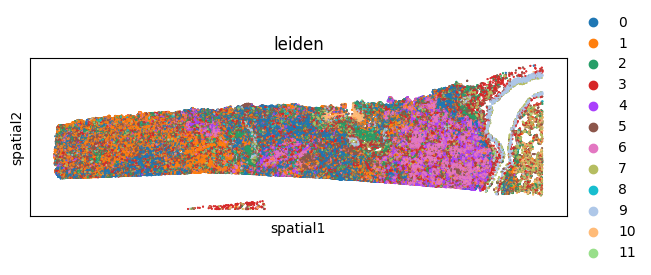
Visualize annotation on UMAP and spatial coordinates:

sc.pl.umap(
    adata,
    color=[
        "total_counts",
        "n_genes_by_counts",
        "leiden",
    ],
    wspace=0.1,
)

sq.pl.spatial_scatter(
    adata,
    library_id="spatial",
    shape=None,
    color=[
        "leiden",
    ],
)

ln.finish()

Show code cell output Hide code cell output

→ finished Run('2Q17Xrf4RXz9E6Cy') after 1m at 2026-01-03 11:53:54 UTC