Interactive visualization using Vitessce 
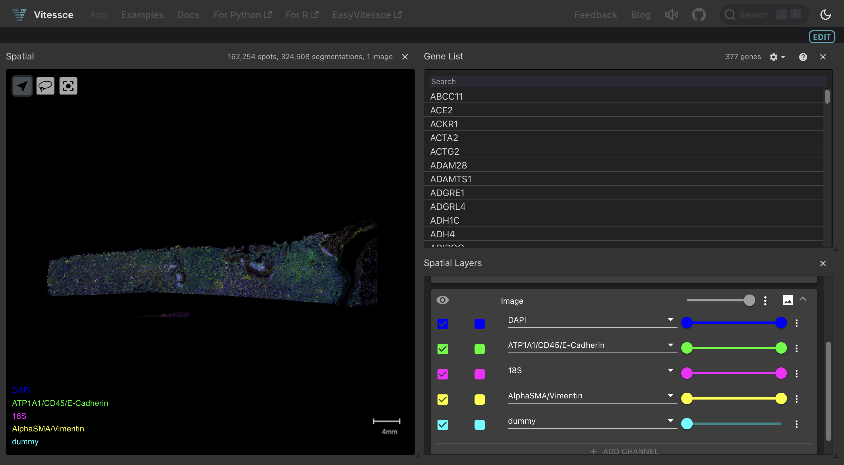
SpatialDatasets can be visualized interactively on LaminHub using Vitessce.
Here is a guide for visualizing spatial data with Vitessce.
This notebook adds the Vitessce visualization to this Xenium dataset discussed on the previous page.