Analyze a collection in memory

Here, we’ll analyze the growing collection by loading it into memory. This is only possible if it’s not too large. If your data is large, you’ll likely want to iterate over the collection to train a model, the topic of the next page ().

import lamindb as ln
import bionty as bt

ln.track("mfWKm8OtAzp8")

Show code cell output Hide code cell output

→ connected lamindb: testuser1/test-scrna

→ created Transform('mfWKm8OtAzp80000', key='scrna4.ipynb'), started new Run('3E74wX4IT9uoXTgS') at 2025-10-30 19:00:33 UTC

→ notebook imports: bionty==1.8.1 lamindb==1.15a1 scanpy==1.11.5

ln.Collection.to_dataframe()

Show code cell output Hide code cell output

	uid	key	description	hash	reference	reference_type	version	is_latest	is_locked	created_at	branch_id	space_id	created_by_id	run_id	meta_artifact_id
id
2	xkEvkoBw2y7KKrmA0001	scrna/collection1	None	luH-jPb6eJLsXvc1TWGpUg	None	None	2	True	False	2025-10-30 19:00:24.978000+00:00	1	1	1	2	None
1	xkEvkoBw2y7KKrmA0000	scrna/collection1	None	DuyXxlMxwF92YehyBLbhKg	None	None	None	False	False	2025-10-30 19:00:06.761000+00:00	1	1	1	1	None

collection = ln.Collection.get(key="scrna/collection1", version="2")

collection.artifacts.to_dataframe()

Show code cell output Hide code cell output

	uid	key	description	suffix	kind	otype	size	hash	n_files	n_observations	version	is_latest	is_locked	created_at	branch_id	space_id	storage_id	run_id	schema_id	created_by_id
id
5	bpbG3gu6O2ljRoT40001	None	10x reference adata, trusted cell type annotation	.h5ad	dataset	AnnData	857336	GK721a-L-fGDI8kXefKMtA	None	70	None	True	False	2025-10-30 19:00:24.480000+00:00	1	1	1	2	NaN	1
1	oTuMP0V231DdGZBx0000	datasets/conde22.h5ad	None	.h5ad	dataset	AnnData	57612943	t_YJQpYrAyAGhs7Ir68zKj	None	1648	None	True	False	2025-10-30 19:00:06.523000+00:00	1	1	1	1	3.0	1

If the collection isn’t too large, we can now load it into memory.

Under-the-hood, the AnnData objects are concatenated during loading.

The amount of time this takes depends on a variety of factors.

If it occurs often, one might consider storing a concatenated version of the collection, rather than the individual pieces.

adata = collection.load()

The default is an outer join during concatenation as in pandas:

adata

Show code cell output Hide code cell output

AnnData object with n_obs × n_vars = 1718 × 36508
    obs: 'donor', 'tissue', 'cell_type', 'assay', 'cell_type_untrusted', 'n_genes', 'percent_mito', 'louvain', 'cell_type_untrusted_original', 'artifact_uid'
    obsm: 'X_umap', 'X_pca'

The AnnData has the reference to the individual artifacts in the .obs annotations:

adata.obs.artifact_uid.cat.categories

Show code cell output Hide code cell output

Index(['oTuMP0V231DdGZBx0000', 'bpbG3gu6O2ljRoT40001'], dtype='object')

We can easily obtain ensemble IDs for gene symbols using the look up object:

genes = bt.Gene.lookup(field="symbol")

genes.itm2b.ensembl_gene_id

Show code cell output Hide code cell output

'ENSG00000136156'

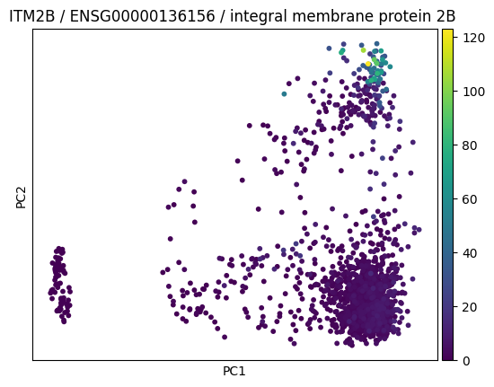
Let us create a plot:

import scanpy as sc

sc.pp.pca(adata, n_comps=2)

sc.pl.pca(
    adata,
    color=genes.itm2b.ensembl_gene_id,
    title=(
        f"{genes.itm2b.symbol} / {genes.itm2b.ensembl_gene_id} /"
        f" {genes.itm2b.description}"
    ),
    save="_itm2b",
)

WARNING: saving figure to file figures/pca_itm2b.pdf

We could save a plot as a pdf and then see it in the flow diagram:

artifact = ln.Artifact(
    "./figures/pca_itm2b.pdf", description="My result on ITM2B"
).save()
artifact.view_lineage()

But given the image is part of the notebook, we can also rely on the report that we create when saving the notebook:

ln.finish()